
An Excel drop down list is a type of data validation tool that lets you select a value from a predefined list, rather than typing it in manually. This is especially useful when you are dealing with frequently repetitive data entry tasks where certain values need to be standardized—such as categories, departments, positions, regions, or product types.
What is excel drop down list?
Creating an Excel drop down list is very easy, and you do not need any coding knowledge for this. You just have to follow a few steps.
First, choose the range of cells and go to the Data tab, then click on Data Validation, and choose the List option; then you enter the item that pop up in the drop-down list. You can also type these values directly, or you can also take them from another sheet or column.
How to Create Excel Drop Down List (From Another Worksheet)
Example
Suppose you have two sheets in your Excel file.
Sheet 1 contains a list of employees
Sheet 2 contains a list of departments
In Sheet 1, you want to assign a department to each employee.
Instead of manually typing the department “Marketing,” “Sales,” “IT,” or “Finance” each time, you can create a drop-down list that will pull the names of departments directly from Sheet 2.


1. Now in the second sheet, type the list of departments that you need to pop up in the dropdown list.

We need to name this list before we can use it for the drop-down.
2. So I will select all the cells that contain the department names. And then I will type a new name by clicking on the name box.

Now you can see the names here.
3. I will select all the cells where I want this dropdown to appear.

4. Then I will click on the Data tab ribbon and choose the Data Validation command.

5. Next, you will see a Data Validation window. In the settings, I will choose “Allow” and then select the list option.

6. I will type an equal sign and the name of the list (department) in the source column.

Let me show you an easier way.
You can press the F3 key on your keyboard, and it will open the “Paste Names” window. I will click on the list I want to use and click “OK,” and now you can see it exactly as we typed it.

7. You will see the Excel drop down list is ready.

Department names are listed in Sheet2
Named range “department” is created
Drop-down is inserted using =department
How to Create Multiple Dependent Excel Drop Down List (Using INDIRECT Function)
Excel provides us with a convenient feature to create multiple dependency drop-down lists in a few easy steps.
For more advanced use, you can create dependent drop down lists—where the second list depends on the first—by using the INDIRECT function and named ranges.
In this example, you want to create two connected excel drop down list.
We have two sheet.
Sheet 1 listing categories like “Fruits” and “Vegetables”

Sheet 2 Containing two columns: Drop Down 1 (Category) and Drop Down 2 (Item Name)

When you select a Category “Fruits” from Drop Down 1, Drop Down 2 should automatically show only fruit options like Apple, Mango, or Banana.

If you select a Category “Vegetables” from Drop Down 1 the second drop-down should switch to Carrot, Spinach, or Potato.

First, we will define a name for each dependency item.
1. I will click on the Formula menu and choose Define Name under the Formula menu.

2. Then select the dependency item cell ranges. Define the category name.
Make sure the name is the same as the category name.

3. Repeat this process for all dependent items in the range.

Now the next step for us is to create the drop-down list.
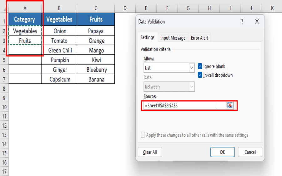
4. First we will create the drop-down list for the Drop Down 1 column using the data validation options.
5. Select the range of cells where you want the dropdown to appear (A2:A12 in our case)

6. In the Source field, we will select the Category column from Sheet1.

7. Next, create the drop-down list for the Drop Down 2 column.
The items should be dependent on the selection of the category items.
8. I will use the INDIRECT function with the source text field.

Result:

Category list: “Fruits” and “Vegetables”
Each list (fruits and vegetables) is named accordingly
Drop-down 1 pulls category
Drop-down 2 uses =INDIRECT(A2) to dynamically show matching list items
Also Read: How to Add Leading Zeros in Excel sheet
Summary:
You can use the Excel drop down list feature by using the Data Validation option. You can create an Excel drop down list by typing the values directly or by referring to a list from another worksheet. It not only saves time but also helps prevent typing errors and keeps your spreadsheet data similar.