
The SUMIFS function in Excel is a powerful tool that allows you to sum values based on multiple conditions. When you are working in Excel and sometimes you come across a condition in which you need to add numbers based on more than one condition. Then at that time SUMIFS function will make your work easy. SUMIFS function is an important tool which provides you the result by totaling the numbers based on more than one criteria given by you.
Through SUMIFS function in Excel you can analyze your data in many ways such as calculating sales, setting sales goals, estimating budgets and counting data. The SUMIFS function in Excel is used to add figures grounded on one or further specific conditions. SUMIFS is the most commonly used function in Excel to perform summation based on conditions. You will find SUMIFS in every type of spreadsheet which calculates conditional sum based on date, text or numbers.
What is the SUMIFS Function in Excel?
The SUMIFS function in Excel adds numbers in a range that meet one or more given criteria.
How to Use SUMIFS function in Excel?
Syntax:
=SUMIFS(sum_range,criteria_range1,criterial,[criteria_range2,criteria2], ...)If you want to know more about SUMIFS function in Excel practice some examples
See the examples given below.
You have multiple products in the given sheet but you want to find out the total sales of printers based on specific region.
Find out the total deals in “west zone” for product “Printer” using SUMIFS formula.
Examples of Sumifs step-by-step.
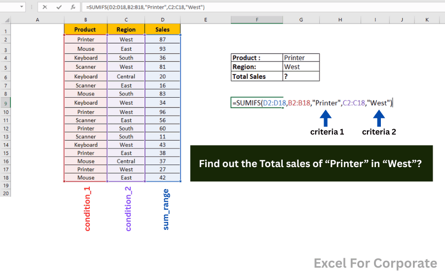
Q. Find out the Total sales of “Printer” in “West”?
Step-by-Step Explanation:
- Select cell and type Sumifs press Tab Key.
- Select sum_range D2:D18 (range from which the total is to be calculated).
- Type ,
- Select range for condition 1, B2:B18
- Type ,
- Criteria 1 “Printer”
- Type ,
- Select range for condition 2, C2:C18
- Type ,
- Criteria 2 “West”
- Close bracket and Hit Enter.

Total 87 + 96 + 27 = 210
Result 210
The SUMIFS function can be used to sum values greater than, less than, and equal to a given range.
Q. Find the total sales of “Printers” whose quantity is more than 20?
Step-by-Step Explanation:
- Select cell and type Sumifs press Tab Key.
- Select sum range E2:E18 (range from which the total is to be calculated).
- Type ,
- Select range for condition 1, B2:B18
- Type ,
- Criteria 1 “Printer.”
- Type ,
- Select range for condition 2, D2:D18
- Type ,
- Criteria 2
">20"(sum value where the quantity is greater than 20). - Close bracket and Hit Enter.

Total 87 + 60 = 147
Result 147
You can use SUMIFS function in Excel, if you need to do calculation grounded on a date. If calculation is to be done between two dates, any specific date, previous date or the sum of the later date.
Q. Find the total sales before 1-Mar-2025.
Formula Used:
=SUMIFS(C2:C12,B2:B12,”<“&E3)
Step-by-Step Explanation:
- Select cell and type Sumifs press Tab Key.
- Select sum range C2:C12 (Sales range from which the total is to be calculated).
- Type ,
- Select range for condition, B2:B12 (Date).
- Type ,
- Criteria “<“&E3 (To sum value before 01-March-2025)
- Close bracket and Hit Enter.

Dates Before 01-Mar-2025:
4-Jan-2025 → 29
10-Jan-2025 → 16
12-Feb-2025 → 25
20-Feb-2025 → 17
22-Feb-2025 → 25
Total 29 + 16 + 25 + 17 + 25 = 112
Result 112
Q. Find the total sales that occurred after 20-Feb-2025.
Formula Used:
=SUMIFS(C2:C12,B2:B12,”>”&E3)
Step-by-Step Explanation:
- Select cell and type Sumifs press Tab Key.
- Select sum range C2:C12 (Sales range from which the total is to be calculated).
- Type ,
- Select range for condition, B2:B12 (Date).
- Type ,
- Criteria “>”&E3 (sum value after 20-Feb-2025)
- Close bracket and Hit Enter.

Dates Greater Than 20-Feb-2025:
22-Feb-2025 → 25
1-Mar-2025 → 25
5-Mar-2025 → 16
10-Mar-2025 → 11
1-Apr-2025 → 15
4-Apr-2025 → 12
15-Apr-2025 → 27
Total = 25 + 25 + 16 + 11 + 15 + 12 + 27 = 131
Result: 131
How to Apply Excel’s SUMIFS with a Date Range (Between Two Dates)
When you are working with Excel, analyzing time-based data is a common task—especially when you want to sum between two given dates using SUMIFS.
Example:
You have a table of sales data by date, and you want to calculate the total sales between 12-Feb-2025 and 1-Mar-2025.
Formula Used:
=SUMIFS(C2:C12,B2:B12,”>=”&E3,B2:B12,”<=”&F3)
Step-by-Step Explanation:
Range Description
C2:C12 sum range — the actual sales values you want to add up.
B2:B12 criteria range — pick out the date column for filter deals.
“>=”&E3 date is larger than or similar to February 12, 2025.
“<=”&F3 date is less than or equal to March 1, 2025.
Sum all values in column C where the corresponding date in column B is between 12-Feb-2025 and 1-Mar-2025.

12-Feb-2025 → 25
20-Feb-2025 → 17
22-Feb-2025 → 25
1-Mar-2025 → 25
Total = 25 +17 + 25 + 25 = 92
How to Use the SUMIFS Function in Excel (Partial Text Match with Wildcards)
(With Wildcards for “Starts With” and “Ends With” Criteria)
In this example, you will learn how to sum values based on partial matches (like product codes that start with “ABC” or end with “00”), the SUMIFS function combined with wildcards becomes a powerful tool.

Example 1: Find the Total Sales where the product code starts with “ABC”.
Formula Used:
=SUMIFS(C2:C11,B2:B11,”ABC*”)
Step by Step Explanation:
Sum Sales Where Product Code Starts with “ABC”
C2:C11 → sum range (“Sales” column).
B2:B11 → criteria range (“Product Code” column).
“ABC*”→the condition. It uses the asterisk * wildcard, which means “starts with ABC”.
This formula looks at each cell in column B (Product Code) and checks if it starts with “ABC”. If it does, it adds the corresponding Sales value from column C.
Matching Entries:
ABC-425 → 100
ABC-355 → 380
ABC-645 → 200
ABC-255 → 378
Total Sales:
100 + 380 + 200 + 378 = 1058
Q2. Find the Total Sales where the product code ends with “00”.
Formula Used:
=SUMIFS(C2:C11,B2:B11,”*00″)
Explanation:
Sum Sales Where Product Code Ends in “00”
“*00” means any text that ends with “00”. The asterisk * allows any number of characters before 00.
Matching Entries:
BEC-500 → 138
XYZ-200 → 216
XYZ-800 → 202
TCE-600 → 168
Total Sales:
138 + 216 + 202 + 168 = 724
You can make a strong filtering option by using SUMIFS from wildcards, even when you are working with text-based codes. If you need to extract totals based on product codes that begin, end, or contain certain strings, SUMIFS function in Excel combined with wildcards you can handle it smartly.
Pro Tips for Using SUMIFS function in Excel
You should use text, numbers and dates for criteria.
When you use dates, make sure that the format in Excel should be correct (avoid text-formatted dates).
You should always use & to combine a with a cell reference, such as “>”&A1.
Verify your data twice consistency in text fields all the time. Your results may be affected through extra spaces or irregular formats.
Conclusion remarks
Anyone using Excel to work with structured data needs to be familiar with the SUMIFS function in Excel. Using a single formula, you can precisely summaries and streamlines intricate filtering.